Bayesian Filters
This module contains Bayesian filters.
All classes from this module are currently imported to top-level pybayes module, so instead of from pybayes.filters import KalmanFilter you can type from pybayes import KalmanFilter.
Filter prototype
- class pybayes.filters.Filter[source]
Abstract prototype of a bayesian filter.
- bayes(yt, cond=None)[source]
Perform approximate or exact bayes rule.
Parameters: - yt (1D numpy.ndarray) – observation at time t
- cond (1D numpy.ndarray) – condition at time t. Exact meaning is defined by each filter
Returns: always returns True (see posterior() to get posterior density)
- posterior()[source]
Return posterior probability density funcion (CPdf).
Returns: posterior density Return type: Pdf Filter implementations may decide to return a reference to their work pdf - it is not safe to modify it in any way, doing so may leave the filter in undefined state.
- evidence_log(yt)[source]
Return the logarithm of evidence function (also known as marginal likelihood) evaluated in point yt.
Parameters: yt (numpy.ndarray) – point which to evaluate the evidence in Return type: double This is typically computed after bayes() with the same observation:
>>> filter.bayes(yt)
>>> log_likelihood = filter.evidence_log(yt)
Kalman Filter
- class pybayes.filters.KalmanFilter(A, B=None, C=None, D=None, Q=None, R=None, state_pdf=None)[source]
Implementation of standard Kalman filter. cond in bayes() is interpreted as control (intervention) input
 to the system.
Kalman filter forms optimal Bayesian solution for the following system:

where
 is hidden state vector,
  is
observation vector and
is
observation vector and  is control vector.
  is normally
distributed zero-mean process noise with covariance matrix
is normally
distributed zero-mean process noise with covariance matrix  ,
,  is normally
distributed zero-mean observation noise with covariance matrix
is normally
distributed zero-mean observation noise with covariance matrix  . Additionally, intial
pdf (state_pdf) has to be Gaussian.
. Additionally, intial
pdf (state_pdf) has to be Gaussian.- __init__(A, B=None, C=None, D=None, Q=None, R=None, state_pdf=None)[source]
Initialise Kalman filter.
Parameters: - A (2D numpy.ndarray) – process model matrix
 from class description
 - B (2D numpy.ndarray) – process control model matrix
 from class description; may be None or unspecified for control-less systems
 - C (2D numpy.ndarray) – observation model matrix
 from class description; must be full-ranked
 - D (2D numpy.ndarray) – observation control model matrix
 from class description; may be None or unspecified for control-less systems
 - Q (2D numpy.ndarray) – process noise covariance matrix from class description; must be positive definite
- R (2D numpy.ndarray) – observation noise covariance matrix from class description; must be positive definite
- state_pdf (GaussPdf) – initial state pdf; this object is referenced and used throughout whole life of KalmanFilter, so it is not safe to reuse state pdf for other purposes
All matrices can be time-varying - you can modify or replace all above stated matrices providing that you don’t change their shape and all constraints still hold. On the other hand, you should not modify state_pdf unless you really know what you are doing.
>>> # initialise control-less Kalman filter:
>>> kf = pb.KalmanFilter(A=np.array([[1.]]),
                         C=np.array([[1.]]),
                         Q=np.array([[0.7]]), R=np.array([[0.3]]),
                         state_pdf=pb.GaussPdf(...))
- A (2D numpy.ndarray) – process model matrix
- bayes(yt, cond=None)[source]
Perform exact bayes rule.
Parameters: - yt (1D numpy.ndarray) – observation at time t
- cond (1D numpy.ndarray) – control (intervention) vector at time t. May be unspecified if the filter is control-less.
Returns: always returns True (see posterior() to get posterior density)
Particle Filter Family
- class pybayes.filters.ParticleFilter(n, init_pdf, p_xt_xtp, p_yt_xt, proposal=None)[source]
Standard particle filter (or SIR filter, SMC method) implementation with resampling and optional support for proposal density.
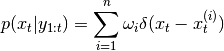
Posterior pdf is represented using EmpPdf and takes following form:
- __init__(n, init_pdf, p_xt_xtp, p_yt_xt, proposal=None)[source]
Initialise particle filter.
Parameters: - n (int) – number of particles
- init_pdf (Pdf) – either EmpPdf instance that will be used directly as a posterior (and should already have initial particles sampled) or any other probability density which initial particles are sampled from
- p_xt_xtp (CPdf) –
 cpdf of state in t given state in t-1
 - p_yt_xt (CPdf) –
 cpdf of observation in t given state in t
 - proposal (Filter) – (optional) a filter whose posterior will be used to sample
particles in bayes() from (and to correct their weights). More specifically,
its bayes
 method is called before sampling
i-th particle. Each call to bayes() should therefore reset any effects of
the previous call.
method is called before sampling
i-th particle. Each call to bayes() should therefore reset any effects of
the previous call.
- bayes(yt, cond=None)[source]
Perform Bayes rule for new measurement
 ; cond is ignored.
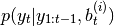
Parameters: cond (numpy.ndarray) – optional condition that is passed to
after  so that is can be rewritten as:
  .
.The algorithm is as follows:
- generate new particles:

- recompute weights:
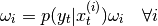
- normalise weights
- resample particles
- generate new particles:
- class pybayes.filters.MarginalizedParticleFilter(n, init_pdf, p_bt_btp, kalman_args, kalman_class=<class 'pybayes.filters.KalmanFilter'>)[source]
Simple marginalized particle filter implementation. Assume that tha state vector
 can be divided into two parts
  and that the pdf representing the process
model can be factorised as follows:
and that the pdf representing the process
model can be factorised as follows:
and that the
 part (given
  ) can be estimated with (a subbclass of) the
KalmanFilter. Such system may be suitable for the marginalized particle filter, whose
posterior pdf takes the form
) can be estimated with (a subbclass of) the
KalmanFilter. Such system may be suitable for the marginalized particle filter, whose
posterior pdf takes the form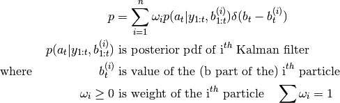
Note: currently
is hard-coded to be process and observation noise covariance of the
part. This will be changed soon and will be passed as condition to
KalmanFilter.bayes().- __init__(n, init_pdf, p_bt_btp, kalman_args, kalman_class=<class 'pybayes.filters.KalmanFilter'>)[source]
Initialise marginalized particle filter.
Parameters: - n (int) – number of particles
- init_pdf (Pdf) – probability density which initial particles are sampled from. (both
and parts)
- p_bt_btp (CPdf) –
 cpdf of the (b part of the) state in t given
state in t-1
cpdf of the (b part of the) state in t given
state in t-1 - kalman_args (dict) – arguments for the Kalman filter, passed as dictionary; state_pdf key should not be speficied as it is supplied by the marginalized particle filter
- kalman_class (class) – class of the filter used for the part of the system;
defaults to KalmanFilter
- bayes(yt, cond=None)[source]
Perform Bayes rule for new measurement
. Uses following algorithm:- generate new b parts of particles:

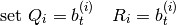 where
where  is
covariance of process (respectively observation) noise in ith Kalman filter.
is
covariance of process (respectively observation) noise in ith Kalman filter.- perform Bayes rule for each Kalman filter using passed observation
- recompute weights:
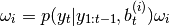 where
where
 is evidence (marginal likelihood) pdf of ith Kalman
filter.
is evidence (marginal likelihood) pdf of ith Kalman
filter. - normalise weights
- resample particles
- generate new b parts of particles: